Adding a drop-down list to a cell in Excel

Let’s say you have created a spreadsheet template that requires input from different users, eg. a sales pipeline for your sales team. In one cell, the input has to be in a very specific manner, eg. months, spelt correctly. Now if left to the different users, there may be typo errors and moreover it doesn’t make sense to have to type an input that’s restricted to some specific list.The answer is to create a drop-down list in that cell for the user to select. That way the spelling will be consistently accurate and not so tedious to type in manually.
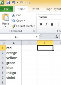
dropdown list 1Step 1:
Create the list in the Excel sheet. In the example, I have created the list of rainbow colours, from A1 to A7, viz. red, orange, yellow, green, blue, indigo, violet.


Step 2:
Select the cell where you want the drop-down list as the input.
I’ve selected cell C1 in the example.
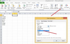
 

data validation 1Step 3:
With Cell C1 still selected, go to the Data menu above, click Data Validation, and again Data Validation from the drop-down menu.


Step 4:
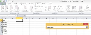
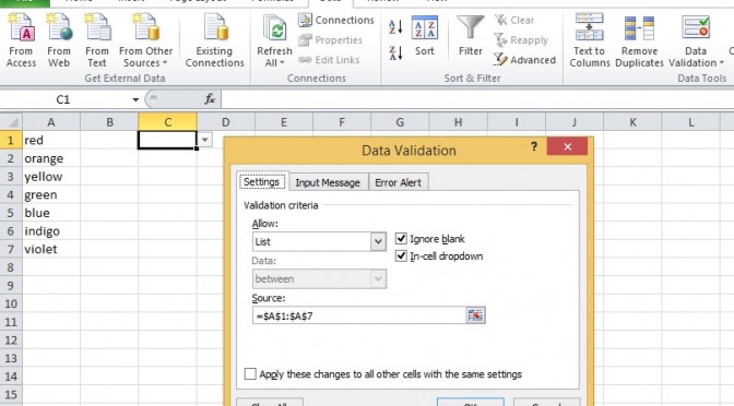
In the box that opens up, choose Settings, Validation criteria, List.
 

data validation 2Step 5:
In the Source selection, click and a new box opens up for Data Validation.
 

dropdown list 2Step 6:
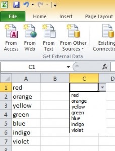
Highlight (select) the list from A1 to A7, enter. Close the Data Validation box, and click OK in the Settings box.
That’s it. Now there’s a little arrow in the cell C1 for your drop-down list of rainbow colours.

How to sort data in Excel

One of the most compelling reasons for having a database is the ability to quickly search or sort the data. But not many people are inclined or able to manage (let alone master) a say SQL Database or even a simple database like Microsoft’s Access (part of the Office Suite).

Well, never fear. If you have used Excel long enough and if you have been creating tables and lists of data in the spreadsheet, you would have felt the need to sort the data alphabetically or by value (largest to smallest, or vice versa). And you can do that easily in Excel!

For example, if you have a contact list that you have been updating as you go along, you would have a mess of a list over time with all the names in no particular order. Wouldn’t it be nice if you can sort that by alphabetical order?

Or how about a list of your travel expenditure when you spent a whole week in Europe and now you have lots of souvenirs that you bought as gifts. You want to sort them by value, from the most expensive to the cheapest, so that you know what to give to who.

OK, let’s see how to sort those two lists.

1. Contacts List

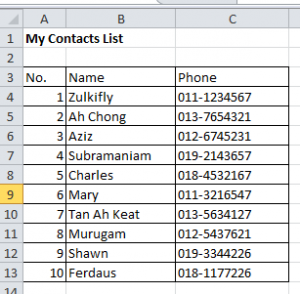
Say you want to sort the names by alphabetical order.

unsorted names


Highlight the cells whose data you want to sort, from B3:C13 (include the header “Name” and “Phone” but not the No. )

sort_contacts

Go to the Home top menu, Sort & Filter at the top extreme right. Click for drop down menu and select Custom Sort.

custom sort

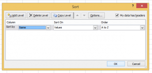
In the Sort Table that opens up, Sort by Column “Name”, Sort on “Values” and Order “A to Z”.

sort

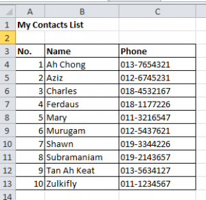
And here’s the sorted Contacts List by names in alphabetical order.

sorted names

2. Travel Shopping List

Similarly for the travel shopping list:

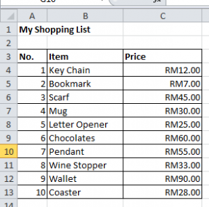
unsorted items

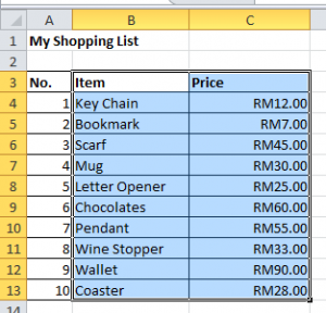
Highlight the cells for the Items and Prices that are to be sorted:

sort_items

Then go to the Home top menu and click on the Sort&Filter for the drop-down menu, select Custom Sort.

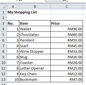
Sort by the Column Price, Value and Order from Largest to Smallest:

sorted prices

Now you know the value from the largest to the smallest, for you to decide the recipients of your gifts.


How to center text across multiple columns in Excel

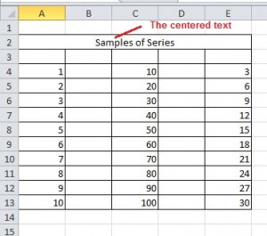
This feature is most useful when you have text in a cell that you use as a label or title for a range. By centering the text across the range, it makes it easier to see that the label or title applies to the entire range.

center text across cells

To center text across multiple columns, do the following:
1. Select a range that consist the text and the cells across which you want to center this text.

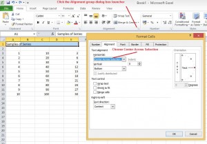
2. On the Home tab, in the Alignment group (or Merge & Center), click the dialog box launcher:

3. In the Format Cells dialog box, on the Alignment tab, click the Horizontal list and then select Center Across Selection in it:
4. Click OK.

centered text

How to number the rows sequentially in Excel

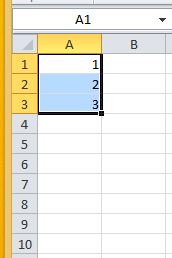
start values
Select the first cell in the range that you want to fill.
Type the starting value for the series.
Type a value in the next cell to establish a pattern. …

Select the cells that contain the starting values.


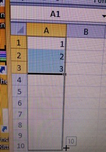
Drag the fill handle across the range that you want to fill.

IMG_8088c filled values


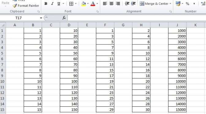
Samples of Series

various values